Pivot Tables in Excel
Pivot tables are one of the most powerful tools in Excel, allowing users to derive meaningful insights from extensive datasets.
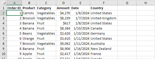
In this example, we have a dataset containing 213 records and six fields: Order ID, Product, Category, Amount, Date, and Country.
💎 Inserting a Pivot Table
Inserting a pivot table is quite easy, just follow these steps:
1. Click on any single cell within the dataset.
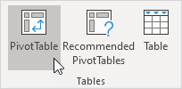
2. Navigate to the Insert tab and, in the Tables group, select PivotTable.
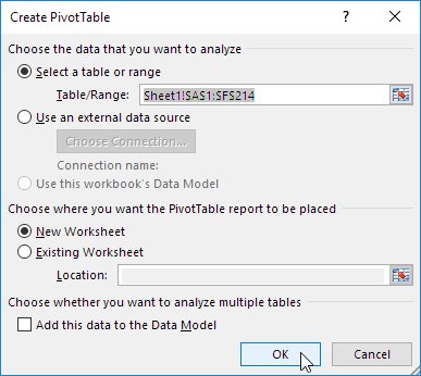
A dialog box will appear, where Excel automatically detects and selects the dataset. By default, the new pivot table will be created in a New Worksheet.
3. Click OK.
💎 Dragging Fields in a Pivot Table
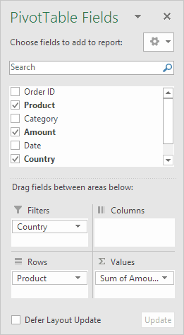
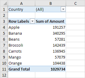
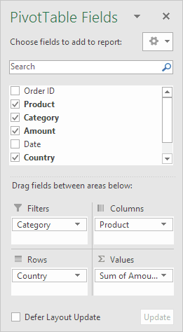
Once the PivotTable Fields pane appears, you can arrange fields in different areas to analyze your data. To calculate the total exported amount for each product:
1. Select the Product field and drag it to the Rows area.
2. Move the Amount field to the Values area.
3. Place the Country field in the Filters area.
The generated pivot table will display a summary of exports, showing that Bananas are the leading export product. This demonstrates how simple and effective pivot tables can be!
💎 Sorting a Pivot Table
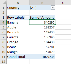
To bring Banana to the top of the list, follow these steps to sort the pivot table:
1. Click on any cell within the Sum of Amount column.
2. Right-click and choose Sort > Sort Largest to Smallest.
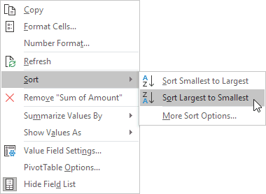
Result: The pivot table is now sorted with the highest values at the top.
💎 Filtering a Pivot Table
Since the Country field has been added to the Filters area, you can filter the pivot table by country. For example, to identify the top exported product to France:
1. Click the filter drop-down and select France.
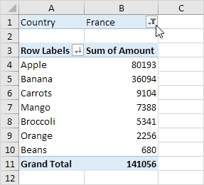
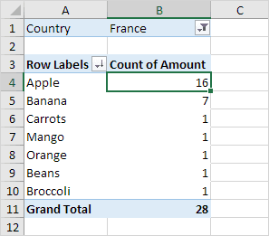
Result: The pivot table will show that Apples are the primary export product to France.
Note: You can also use the standard filter (click the small triangle next to Row Labels) to display only specific product amounts.
💎 Changing the Summary Calculation
By default, Excel summarizes numerical data using either a sum or a count function. To modify this calculation method:
1. Click on any cell inside the Sum of Amount column.
2. Right-click and select Value Field Settings.
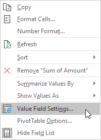
3. Choose the desired calculation type (e.g., select Count).
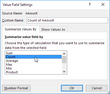
4. Click OK.
Result: The table updates to show that 16 out of 28 orders to France consisted of Apples.
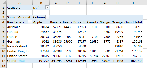
💎 Creating a Two-Dimensional Pivot Table
By assigning fields to both the Rows and Columns areas, you can generate a two-dimensional pivot table. Follow these steps:
1. Move the Country field to the Rows area.
2. Select the Product field and drag it to the Columns area.
3. Place the Amount field in the Values area.
4. Add the Category field to the Filters area.
Result: The two-dimensional pivot table displays total exports for each product across different countries.
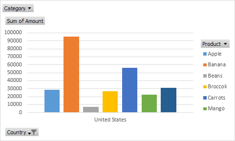
💎 Creating a Pivot Chart
To visually compare data more effectively, create a Pivot Chart and apply filters. While this may seem advanced at this stage, it showcases one of the many powerful capabilities of pivot tables in Excel.
✅ 1/9 Completed! Learn more about pivot tables ➝
Next Chapter: Tables
Other Resources
Microsoft Excel Pivot Table For Beginners - A Step-by-Step Guide
To Master Excel Pivot Table Made Easy
Excel 2024 Pivot Tables Including The Smart Data Model - PDF Book