Filter Data in Excel
Learn how to filter your Excel data to display the records that match specific criteria. This is the first lesson in our in-depth 10-part filtering course.
1. Select any single cell within your data set.
2. Navigate to the Data tab, and in the Sort & Filter group, click Filter.
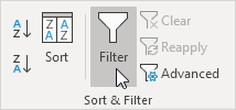
Excel will add drop-down arrows to the column headers.

3. Click on the arrow in the Country column.
4. Uncheck Select All, then check the box next to USA.
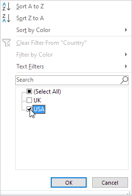
5. Click OK.
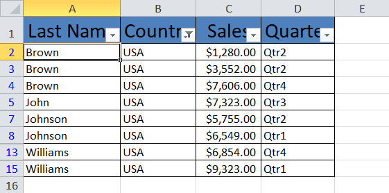
Result: Excel will now display only the sales records from the USA.
6. Click the arrow next to Quarter.
7. Click Select All to clear all checkboxes, then select Qtr2.
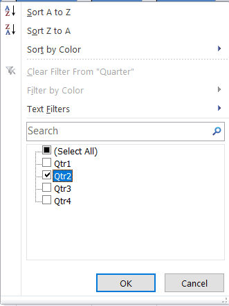
8. Click OK.
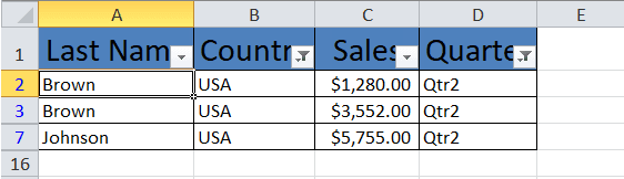
Result: Excel will now show only the sales records from the USA for Qtr2.
9. To remove the filter, go to the Data tab, and in the Sort & Filter group, click Clear. To remove both the filter and the arrows, click Filter again.
![]()
A Faster Way to Filter Data
1. Select a cell in the column you want to filter.

2. Right-click and choose Filter > Filter by Selected Cell’s Value.
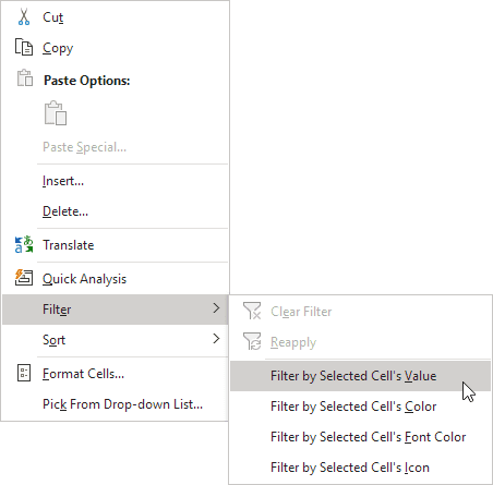
Result: Excel will instantly filter the data to show only records that match the selected value. In our case, Excel will show the sales in the USA.
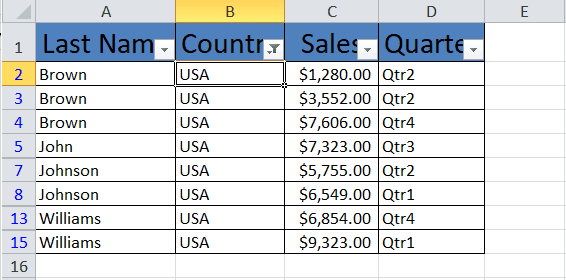
Note: To refine your filtering further, simply select another cell in a different column and apply an additional filter on this data set.
✅ Lesson 1 of 10 completed! Continue learning about filtering in Excel ➝
Next Chapter: Conditional Formatting