Excel Lookup & Reference Functions
These are the functions mostly used when you work with real-world data. Here we will discuss some of the most important lookup function like VLOOKUP, HLOOKUP, INDEX, MATCH, and CHOOSE.
VLOOKUP formula in Excel
VLOOKUP always searches the value in the first column of the table to match the search value. IF the value is match then it returns a corresponding value from a different column (as mention by you) in that row.
1. Insert the VLOOKUP function shown below.
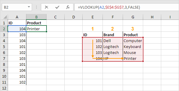
Explanation: This function searches for ID (104) in the selected cell from E4 to G7. Once found, it retrieves the value from the third column of that row. The last part of the formula is set to FALSE to make sure it finds an exact match. If the ID does not exist, the system will display a #N/A error.
2. Select the cell B2 and drag it down to cell B11.
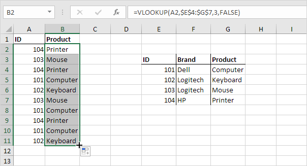
Note: When you copy the VLOOKUP formula downward, the fixed reference ($E$4:$G$7) does not change, but the relative reference (A2) becomes A3, A4, A5, and so on. You can find more details and examples on our VLOOKUP function page.
Excel formula HLOOKUP
In the same way, HLOOKUP finds informexcel formula vlookup and hlookupation in horizontal rows.
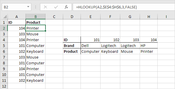
Note: With Excel 365 or Excel 2021, the XLOOKUP function allows you to search across rows using a horizontal lookup.
Excel formula MATCH
The MATCH function gives the number that tells where a certain value appears in a range.
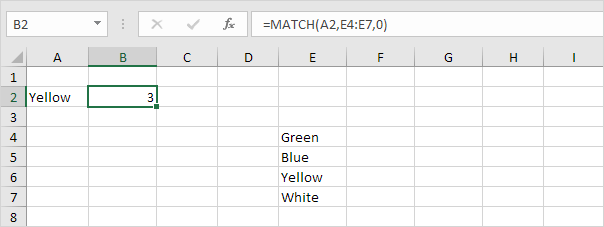
Explanation: The function outputs the number 3, as “yellow” is present at the third position in the range E4:E7. It is not essential to include the third argument when using the MATCH function. Enter zero (0) to find the exact match of the value as in cell A2. IF a match is not found, it will return a #N/A error.
INDEX
The INDEX function is used here to get a value from a two-dimensional range using row and column numbers.
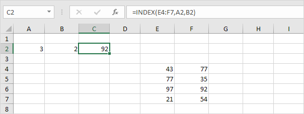
Explanation: Within the range E4:F7, the value 92 appears at the point where row 3 crosses column 2.
Using the INDEX function, you get a value from a one-dimensional range according to its place.
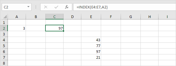
Explanation: 97 is found at position three inside the range E4 to E7. INDEX and MATCH functions are more efficient for finding data.
CHOOSE
Use the CHOOSE function to get a value from a list of items using a position number.
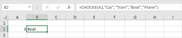
Explanation: The Boat was found at position 3.
1/15 Completed! More about lookup & reference ➝
Next Chapter: Financial Functions
Leave a Reply