Cell References in Excel
Cell references in Excel are very important. Knowing the difference between relative, absolute, and mixed references in Excel is useful.
Relative Reference
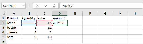
By default, Excel uses relative references. See the formula in cell D2 below. Cell D2 is point (referenced) to cells B2 and C2, meaning its result depends on them. Both references are relative.
1. Select cell D2. Hover your cursor over the small box in the bottom-right corner. When the cursor becomes a plus sign, click and drag it down to cell D5.
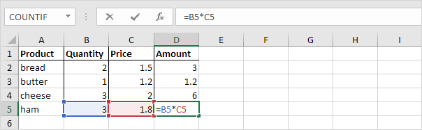
Cell D3 references cell B3 and cell C3. Cell D4 references the values in cells B4 and C4. Cell D5 refers to cell B5 and cell C5. This means each cell references the two cells immediately before it in the same row.
Absolute Reference
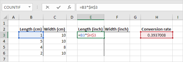
See the formula in cell E3 below.
1. In cell E3, enter $H$3 in the formula to make sure the cell reference stays constant (absolute reference) when copying it to other cells. The $ symbols lock both the column and row.
2. It is now easy to use this formula in the other cells by dragging it.
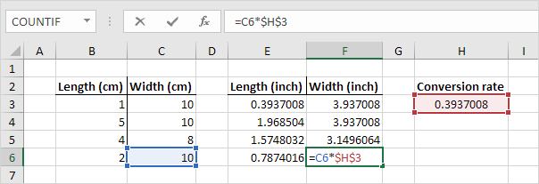
The cell reference H3 is locked, so when the formula is copied down or across, it still uses the correct value. This allows you to get the correct measurements in inches for length and width. To learn more, visit our page on absolute references.
Mixed Reference
It is common to use both relative and absolute references together in some cases. This is called a mixed reference.
1. Check the formula shown in cell F2.
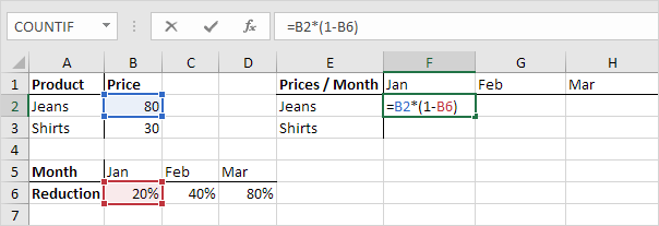
2. To move the formula from cell F2 to the next cell, drag the small square at the bottom-right corner of the cell one cell to the right. Take a moment to review the formula in cell G2.
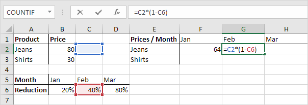
Do you see what happens? Column B should always be used as the reference for the price. To do this, add a dollar sign ($) before the column letter in the formula, like this: $B2 in cell F2.
In the same way, when copying the formula down from cell F2, make sure the reference to the reduction always refers to row 6. To fix this, add a dollar sign ($) before the row number, like this: B$6 in the formula.
Result:
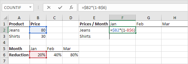
Note: We do not put a $ sign before the row number in $B2. This makes the row number change from 2 (Jeans) to 3 (Shirts) when the formula is copied down. Similarly, we do not put a $ sign before the column letter in B$6. This allows the column letter to change from B (January) to C (February) and D (March) when you copy the formula across the cells.
3. Now, we can easily copy this formula to the other cells by dragging it.
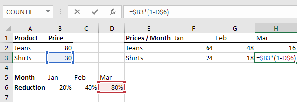
The reference to column B and row 6 is locked, so it will not change when copied or moved.
1/11 Completed! Want to know more about cell references? ➝
Next Chapter: Date & Time Functions