Conditional Formatting in Excel
One of the best uses of Excel’s conditional formatting is to highlight cells based on the cell content automatically. You can apply pre-set rules or custom formulas to determine which cells should be formatted.
Highlight Cells Rules
To highlight cells that contain values greater than a specific number, follow these steps:
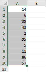
1. Select the range A1:A10.
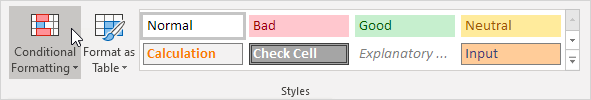
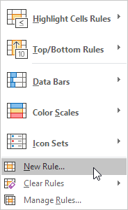
2. From the Home tab, click on Conditional Formatting in the Styles group.
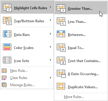
3. Choose Highlight Cells Rules and Greater Than.
4. Enter a value, let’s say 80, and choose a formatting style.

5. Click OK.
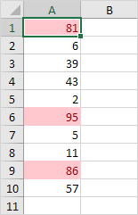
Result: Excel highlights all cells containing values greater than 80.

6. Modify the value in cell A1 to 81.
Result: Excel automatically updates the formatting for cell A1.
Note: You can also use this option (step 3) to highlight cells that contain values less than a specific number, values between two numbers, exact matches, specific text, date-based values (such as today, last week, next month), duplicate entries, or unique values.
Clear Conditional Formatting Rules
To remove a conditional formatting rule, follow these steps:
1. Select the range A1:A10.

2. From the Home tab, select Conditional Formatting in the Styles group.
3. Choose Clear Rules, then click Clear Rules from Selected Cells.
![]()
Top/Bottom Rules
Follow these steps to highlight values that are above average:
1. Select the range A1:A10.

2. From the Home tab, select Conditional Formatting in the Styles group.
3. Select Top/Bottom Rules, then choose Above Average.

4. Pick a formatting style.

5. Click OK.
Result: Excel calculates the average (e.g., 42.5) and highlights cells with values exceeding this average.

Note: This feature (step 3) can also be used to highlight the top n values, top n%, bottom n values, bottom n%, or values below the average.
Conditional Formatting with Formulas
Enhance your Excel skills by using formulas to decide which cells to format. The formulas used for conditional formatting should return TRUE or FALSE.
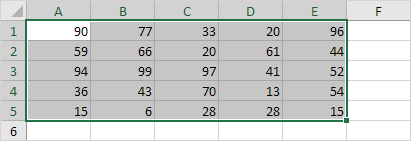
1. Select the range A1:E5.
2. From the Home tab, click on Conditional Formatting in the Styles group.
3. Click New Rule.
4. Then choose Use a formula to determine which cells to format.
5. Enter the formula =ISODD(A1).
6. Choose a formatting style and click OK.

Result: Excel highlights all odd numbers.

Explanation: The formula should be written for the top-left cell of the selected range. Excel then applies the formula automatically to the rest of the cells. For example, cell A2 will use the formula =ISODD(A2), cell A3 will use =ISODD(A3), and so on.
Here’s another example:
7. Select the range A2:D7.

8. Repeat steps 2-4.
9. Enter the formula =$C2=”USA”.
10. Choose a formatting style and click OK.

Result: Excel highlights all records where the country is the USA.
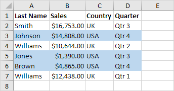
Explanation: The $ symbol locks column C, ensuring that the condition applies across all corresponding rows. For example, cells B2, C2, and D2 will use the formula =$C2=”USA”, while cells A3, B3, C3, and D3 will use =$C3=”USA”, and so on.
Color Scales
Color scales allow you to apply different colors to different values, making it easier to identify high and low points in your dataset.

Tip: Explore how to use color scales effectively to create a heat map.
Highlighting Blank Cells
Conditional formatting can also be used to highlight blank cells, helping to ensure data completeness and making missing information easily noticeable.
![]()
Tip: Discover how to highlight blank cells on our dedicated page about blanks.
✅ 1/10 Completed! Learn more about conditional formatting ➝
Next Chapter: Charts