Transpose Data in Excel
The Transpose feature under Paste Special in Excel allows you to switch data from rows to columns or from columns to rows. You can also use the TRANSPOSE function.
💎 Paste Special Transpose
To transpose data, execute the following steps.
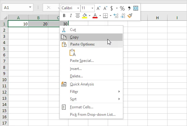
1. Select the range A1:C1.
2. Right-click, and then click Copy.
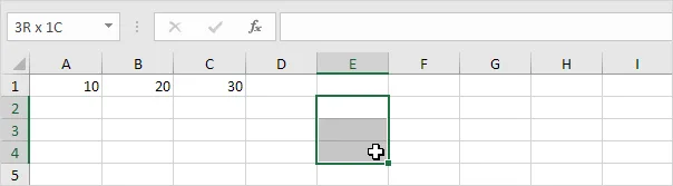
3. Select cell E2.
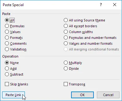
4. Right-click, and then click Paste Special.
5. Check Transpose.
![]()
6. Click OK.
![]()
💎 Excel TRANSPOSE function
Follow these steps to insert the TRANSPOSE function.
1. First, select the new range of cells.
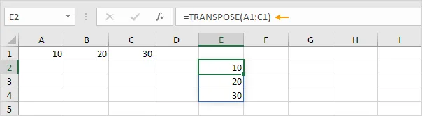
2. Type in =TRANSPOSE(
3. Choose the range A1 to C1, and complete the formula with a closing parenthesis.
![]()
4. To finish, hold CTRL and SHIFT, then press ENTER.
![]()
Note: When you see curly braces {} in the formula bar, it means the formula is an array formula. To remove this array formula, highlight the cells E2 to E4 and press the Delete key.
5. If you are using Excel 365 or Excel 2021, click on cell E2, type the TRANSPOSE function, and then press Enter. Bye bye curly braces.
Note: When you use the TRANSPOSE function in cell E2, it spreads the result across several cells. Wow! This behavior in Excel 365/2021 is called spilling.
💎 Transpose Table without Zeros
When you use the TRANSPOSE function in Excel, any blank cells become zeros. You can resolve this problem by using the IF function.
1. For example, cell B4 below is blank. Using the TRANSPOSE function, the blank cell becomes zero in cell G3.
![]()
2. If the cell is blank, the IF function below gives an empty value (shown as two double quotes “”) to transpose.
![]()
💎 Transpose Magic
Using ‘Paste Special Transpose’ is an effective way to rearrange data from rows to columns or vice versa. However, to maintain a link between the source and target cells, you need some special tricks.
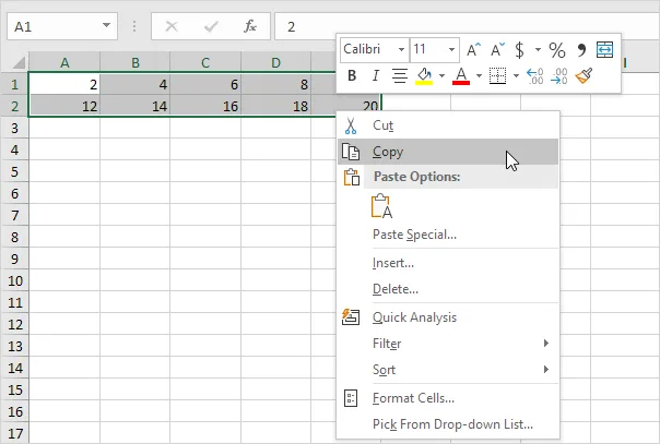
1. Select the range A1:E2.
2. Right-click, and then click Copy.
3. Select cell A4.
4. Right-click, and then click Paste Special.
5. Click Paste Link.
Result:
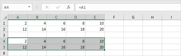
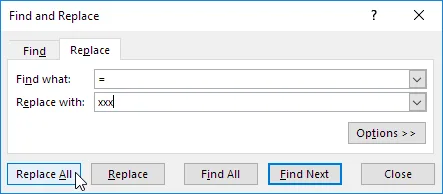
6. Highlight the range A4:E5, then replace every equal sign (=) with xxx.
Result:
![]()
7. To rearrange this data from rows to columns or columns to rows, use ‘Paste Special’ and then choose ‘Transpose’.
![]()
8. Select the cells from G1 to H5 and replace every ‘xxx’ with an equal sign, reversing step 6.
![]()
Note: for example, update cell C2 by changing its value from 16 to 36. The number in cell H3 will be updated from 16 to 36.
8/12 Completed! Learn much more about ranges ➝
Next Chapter: Formulas and Functions