Multi-level Pivot Table in Excel
A PivotTable allows you to include multiple fields in the same area. We will look at an example that includes multiple row fields, multiple value fields, and multiple report filter fields.
We are working with a dataset that contains 213 records and 6 fields: order ID, Product, Category, Amount, Date and Country.

💎 Multiple Row Fields
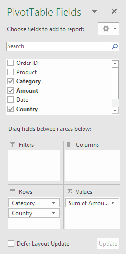
First, insert a pivot table. Next, move these fields to the different areas as shown.
1. Move the Category and Country fields to the Rows area.
2. Amount field to the Values area.
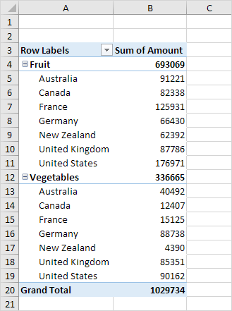
Below you can find the multi-level pivot table.
💎 Multiple Value Fields
First, insert a pivot table. Next, move the following fields to the specified areas.
1. Country field to the Rows area.
2. Amount field to the Values area (2x).
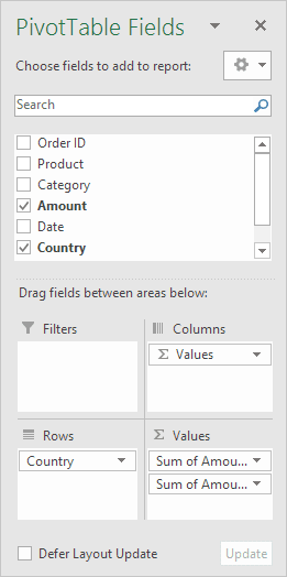
Note: When you drag the Amount field to the Values area a second time, Excel automatically adds it to the Columns area as well.
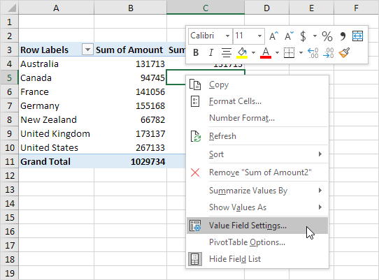
Pivot table:

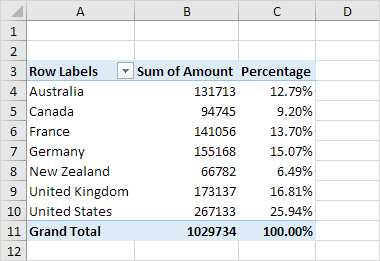
3. Next, click on any cell in the “Sum of Amount2” column.
4. Right-click the field, then choose Value Field Settings from the menu.
5. Enter Percentage for Custom Name.
6. Under the Show Values As tab, select the option % of Grand Total.

7. Click OK.
Result:
💎 Multiple Report Filter Fields
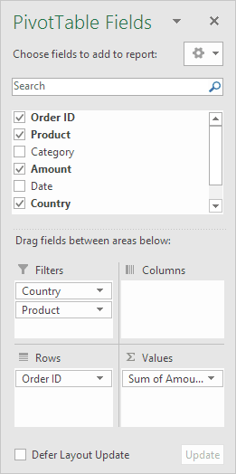
First, insert a pivot table. Now, drag the fields below into the different sections.
1. Order ID to the Rows area.
2. Amount field to the Values area.
3. Move the Country field and the Product field into the Filters area.
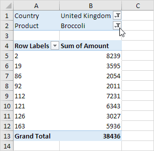
4. Next, choose the United Kingdom from the first drop-down and Broccoli from the second drop-down.
In the pivot table, you can see all ‘Broccoli’ orders for the United Kingdom.
3/9 Completed! Learn much more about pivot tables ➝
Next Chapter: Tables