Group Pivot Table Items in Excel
Follow this example to learn how to group pivot table items in Excel. Understand how to categorize products and arrange dates by quarters.
Below you can find a pivot table. Go back to the Pivot Tables tutorial to understand how to make this pivot table.

💎 Group Products (group data in pivot table)
The Product field contains 7 items. Apple, Banana, Beans, Broccoli, Carrots, Mango and Orange.
To create two groups, execute the following steps.
1. Within the pivot table, select the items Apple and Banana.
2. Right-click and click on Group.
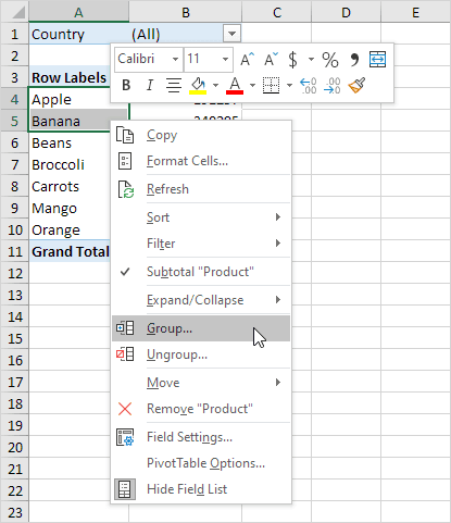
3. From the pivot table, click on Beans, Broccoli, Carrots, Mango, and Orange to select them.
4. Right-click and click on Group.
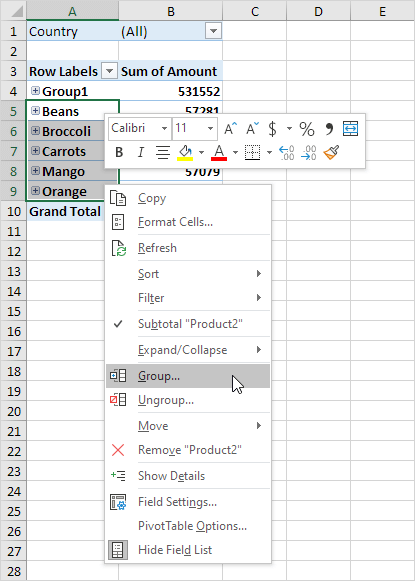
Result:
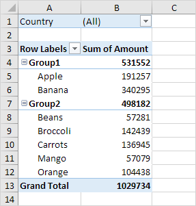
Note: To rename a group (Group1 or Group2), click the group name and type the new name in the formula bar. To remove a group, select it, right-click, and select the ‘Ungroup’ option.
5. To collapse the grouped items, select the corresponding minus signs.
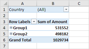
Conclusion: The combined total of Apple and Banana (Group 1) is greater than the total of all products in Group 2.
💎 Group Dates
To create the pivot table shown below, add the Date field to the Rows area in place of the Product field. The Date field contains many items. 6-Jan, 7-Jan, 8-Jan, 10-Jan, 11-Jan, etc.
To categorize the dates by quarters, execute the steps below.
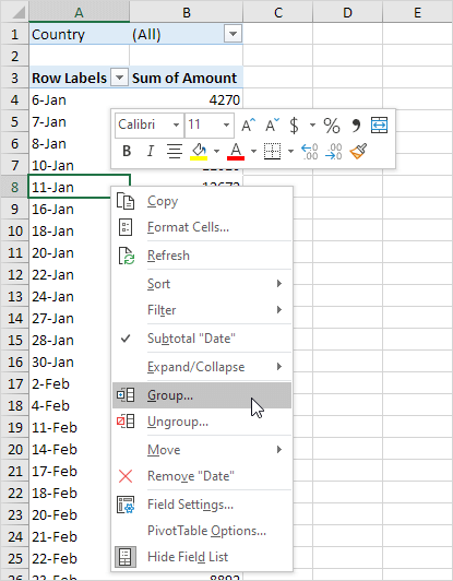
1. Select any cell within the column containing dates.
2. Right-click and click on Group.
3. Select Quarters and click OK.
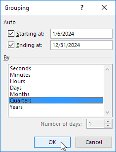
Note: You can also choose to group data by seconds, minutes, hours, and so on.
Result:
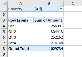
Conclusion: Quarter 2 is the best quarter.
2/9 Completed! Learn much more about pivot tables ➝
Next Chapter: Tables