Dynamic Arrays in Excel
Dynamic Arrays in Excel is a special feature introduced in Excel 365 and Excel 2021. A dynamic array formula entered in one cell automatically fills multiple cells. This behavior in Excel 365/2021 is called spilling. It reduces the need for complex formulas and manual adjustments, making data analysis simpler.
💎 Formula Example
Let’s start with an easy example.
1. Add a $ before the column letter and row number to lock the reference to cell E2.
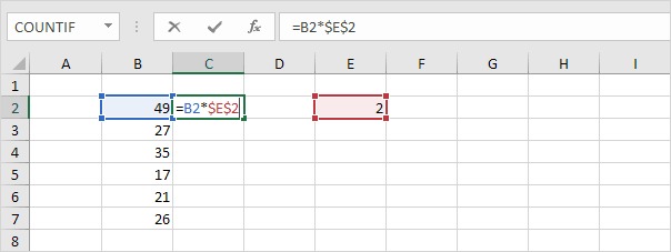
2. Select cell C2, click and hold the small square at its bottom-right corner, and drag it down to C7 to copy the formula.
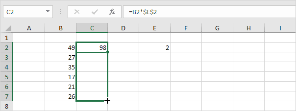
Check:
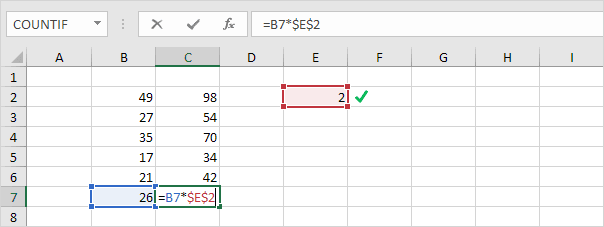
Explanation: The absolute reference ($E$2) does not change, while the relative reference (B2) updates to B3, B4, B5, B6, and B7.
3. If you are using Excel 365 or Excel 2021, enter the formula below in cell C2.
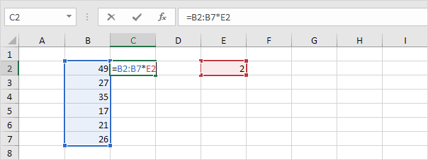
4. Press Enter.
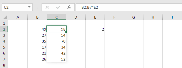
Explanation: This dynamic array (DA) formula, used in cell C2, fills multiple cells at once. This behavior in Excel 365/2021 is called spilling. When you click on a cell in the range C2 to C7, a blue border will appear.
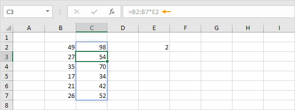
5. When you select a cell between C3 and C7, the formula bar will display the formula in grey.
💎 Dynamic Array Functions
Excel 365 and Excel 2021 offer many new functions for dynamic arrays. To know more about these functions, follow the links given below.
1. The SORT function here sorts the data by the second column in increasing order.
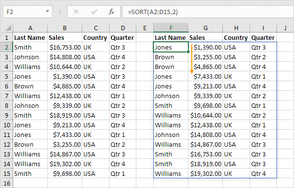
Note: The dynamic array function in cell F2 returns results into several cells. Wow!
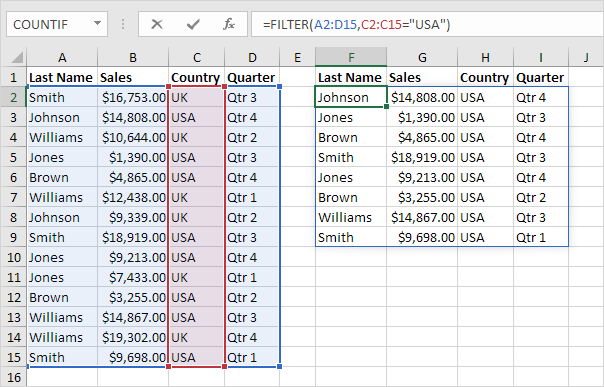
2. The FILTER function below selects only the records from the USA.
3. The RANDARRAY function generates random decimal values within the range of 0 to 1. The array shown below has 5 rows and 2 columns.

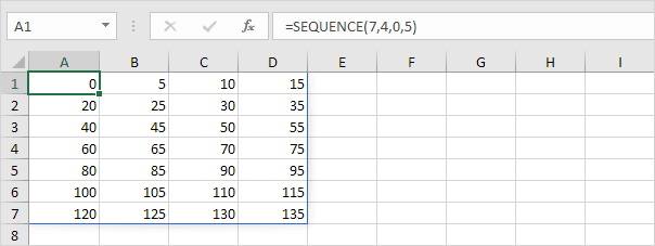
4. This SEQUENCE function generates an array that has 7 rows and 4 columns. The numbers start at 0 and increase by 5 for each new value.
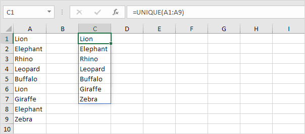
5. The UNIQUE function, by default, shows the unique values from the range.
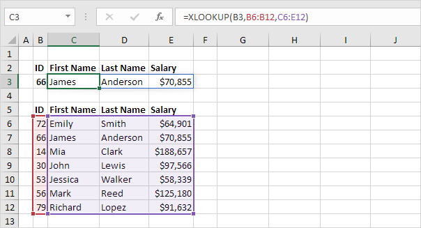
6. The XLOOKUP function in this example identifies the ID and retrieves the matching first name, last name, and salary.
Note: For Excel 365 or Excel 2021 users, choose XLOOKUP in place of VLOOKUP. The XLOOKUP function is user-friendly and includes additional features.
7. The SORTBY function helps you sort data by referring to values from another range.
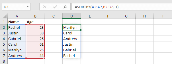
Note: Choose 1 for ascending sorting and -1 for descending sorting.
💎 Old Array Formulas
Old array formulas still work. The good news is that in Excel 365 and Excel 2021, the CTRL + SHIFT + ENTER shortcut is no longer required. Below you can find a few examples.
1. You enter a traditional array formula by pressing CTRL + SHIFT + ENTER.
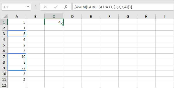
Explanation: This formula sums the 4 largest numbers.
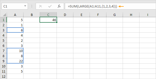
2. In Excel 365/2021, you can complete the formula by just pressing Enter. Bye-bye curly braces.
3. To use the traditional TRANSPOSE function, select the range E2:E4 and press CTRL + SHIFT + ENTER to execute it.

Explanation: The TRANSPOSE function changes a row of data into a column, or a column into a row. The same also applies to ranges.
4. Typing this function in one cell in Excel 365/2021 automatically fills the neighboring cells with results.

💎 Spill Range
Use the first cell and a hash (#) to reference all the values in the blue rectangle, known as the spill range.
1. For example, the UNIQUE function used in cell C1 will list only the unique values.

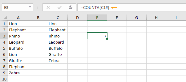
2. The COUNTA function below counts unique values using the spill range C1#.
3. Excel shows the #SPILL! Error if a formula cannot fill the required cells.
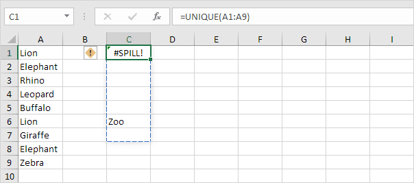
Note: To correct the #SPILL! error, make sure cell C6 is empty.
9/13 Completed! Learn much more about array formulas ➝
Next Chapter: Sort