Drop-down List in Excel
A drop-down list in Excel is useful when you want users to choose from specific options, making sure they do not enter other values.
💎 Create a Drop-down List
Follow these steps as described below:
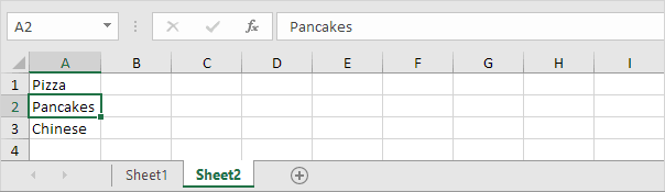
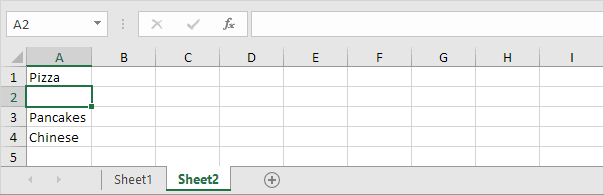
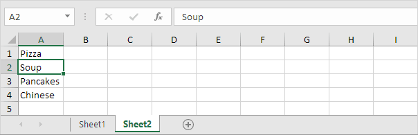
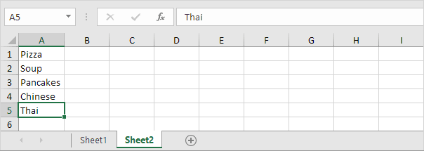
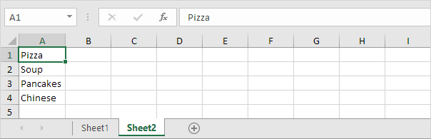
1. Write all drop-down items on sheet 2.
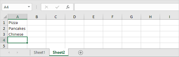
Note: To stop users from accessing Sheet2, you can hide it. Right-click the Sheet2 tab and choose Hide to make it invisible.
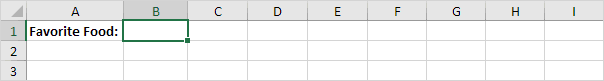
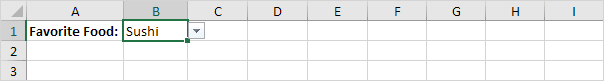
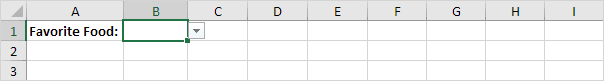
2. On the first sheet, select cell B1.
3. First, go to the Data tab. Now choose “Data Validation” from the Data Tools option.
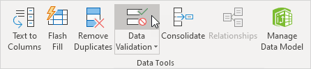
The ‘Data Validation’ dialog box appears.
4. In the Allow box, click List.
5. Inside the Data Validation window, click on the Source option. Now, select the range A1:A3 from Sheet2.
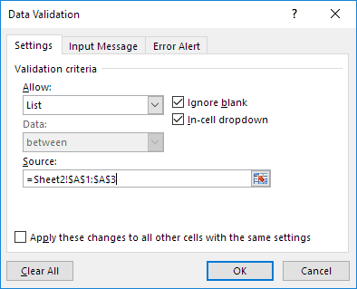
6. Click OK.
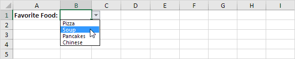
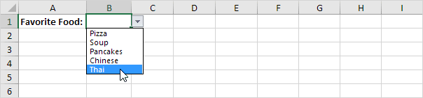
Result:
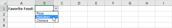
Note: To copy the drop-down list, simply click the cell and press CTRL + C to copy. Choose a new cell, and use CTRL + V to paste the copied data.
7. You can enter the items manually in the Source box rather than selecting a cell range.
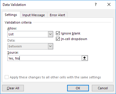
Note: this makes your drop-down list case sensitive. For example, if you input “yes,” it displays an error message.
💎 Allow Other Entries
In Excel, you can make a drop-down menu that accepts both listed and custom entries.
1. Excel shows an error if you type a value that does not match the list.
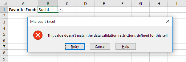
To allow other entries, execute the following steps.
2. First, go to the Data tab. Now choose “Data Validation” from the Data Tools option.
The ‘Data Validation’ dialog box appears.
3. In the Error Alert tab, turn off the option “Show error alert after invalid data is entered” by removing the checkmark.
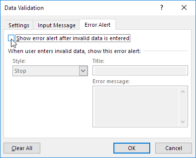
4. Click OK.
5. The list now allows values that are not already listed.
💎 Add/Remove Items
You can easily change the contents of a drop-down list in Excel without opening the ‘Data Validation’ window. This saves time.
To add an item to the list:
1. First, select an item from the list.
2. Right-click, and then click Insert.
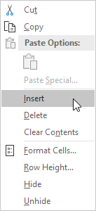
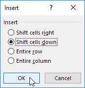
3. Select “Shift cells down” and click OK.
Result:
Note: Excel updated the range from Sheet2!$A$1:$A$3 to Sheet2!$A$1:$A$4 on its own. To check, open the Data Validation dialog box.
4. Type a new item.
Result:
5. To remove an item from the list, do the following: In step 2 above, select the Delete option instead of Insert. Then select Shift cells up and press OK.
💎 Dynamic Drop-down List
You can set up a formula so that your drop-down list updates itself when new items are added.
1. On the first sheet, select cell B1.
2. Now, go to the Data tab. Then, from the Data Tools option, choose “Data Validation”.
The ‘Data Validation’ dialog box appears.
3. In the Allow box, click List.
4. Go to the Source box and write the formula given below.
=OFFSET(Sheet2!$A$1,0,0,COUNTA(Sheet2!$A:$A),1)
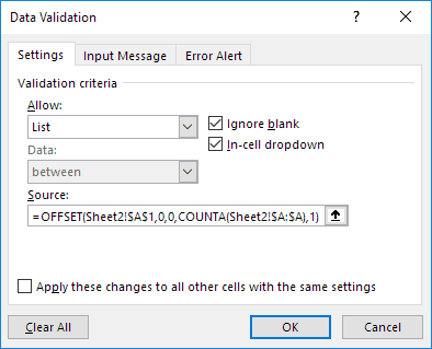
Explanation: The OFFSET function uses five arguments. Here, the reference is Sheet2!$A$1, with 0 rows and 0 columns to move. The height is set as COUNTA(Sheet2!$A:$A) and the width as 1. The COUNTA function is used to count the cells which is not empty in column A of Sheet2. Whenever you input a new item on Sheet2, the COUNTA(Sheet2!$A:$A) value increases. Therefore, the OFFSET function returns a bigger range, which updates the drop-down list.
5. Click OK.
6. Add a new item to the bottom of the list on sheet two.
Result:
💎 Remove a Drop-down list in Excel
Steps to delete a drop-down list in Excel.
1. Select the cell with the drop-down list.
2. Now, go to the Data tab. Then from the Data Tools option, choose “Data Validation”.
The ‘Data Validation’ dialog box appears.
3. Click Clear All.
![]()
Note: It is possible to delete all drop-downs with the same settings. You can do this by selecting the option “Apply these changes to all other cells with the same settings”. And then click the Clear All option.
4. Click OK.
💎 Dependent Drop-down Lists
Do you wish to know more about creating drop-down lists in Excel? Learn how to create dependent drop-down lists.
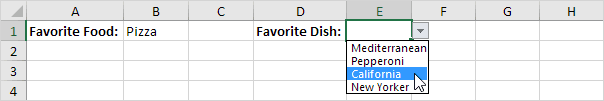
1. As an example, if Pizza is selected from the first drop-down menu.
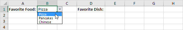
2. A second drop-down displays all the available Pizza items.
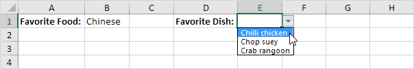
3. If “Chinese” is selected from the first list, the second list automatically display the list of Chinese dishes.
💎 Table Magic
You can use an Excel table to create a drop-down list and automatically update the table item from the table.
1. Select an item as shown below.
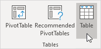
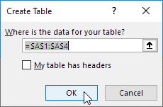
2. Click the Insert tab, look for the Tables group, and choose Table.
3. Excel automatically selects the data for you. Click OK.
4. When you select the list, Excel will show the structured reference automatically.
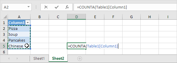
5. You can use this structured reference to create a drop-down list that updates on its own.
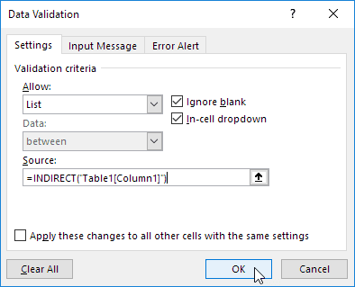
Explanation: The INDIRECT function turns text into a valid reference for cells or ranges.
6. On sheet two, add one more item to the bottom of the list.
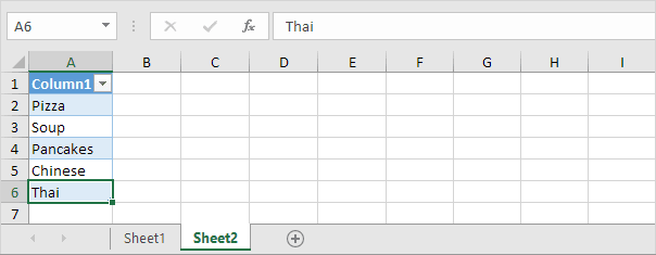
Result:
Note: Try it yourself. Get the attached example file and try to create the list.
7. Use UNIQUE to get a list of unique items in Excel 365 or 2021.
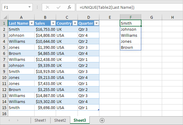
Note: The dynamic array function in cell F1 produces values that fill multiple cells. This behaviour in Excel 365/2021 is called spilling.
8. Create a drop-down list using this spill range.
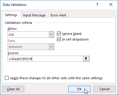
Explanation: To access a spill range, use the first cell along with the # symbol.
Result:
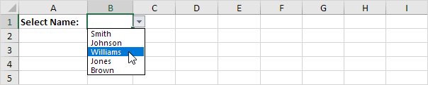
Note: The UNIQUE function shows only distinct values, and Excel automatically refreshes the drop-down list when the data changes.
6/9 Completed! Learn much more about data validation ➝
Next Chapter: Keyboard Shortcuts