Find Duplicates in Excel
On this page, you will learn how to identify duplicate or triplicate values and duplicate rows in Excel. It also explains the steps to eliminate duplicates by using the Remove Duplicates option.
💎 Find Duplicate Values in Excel
Steps to highlight duplicate values in Excel.
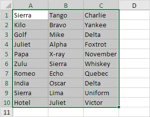
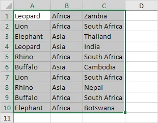
1. Select the range A1:C10.
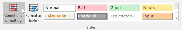
2. First, go to the Home tab and look for the Styles section. Then, click on Conditional Formatting.
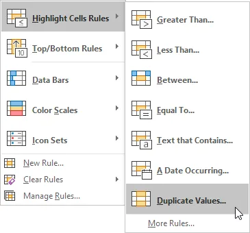
3. Click Highlight Cells Rules, Duplicate Values.
4. Select a formatting style and click OK.
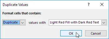
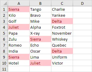
Result: Excel highlights the duplicate names.
Note: Choose Unique in the first drop-down menu to show only unique names.
💎 Find Triplicates
Excel automatically highlights repeated values, including duplicates like Juliet and Delta, and triplicates like Sierra. (see previous image). Execute the following steps to highlight triplicates only.
1. First, clear the previous conditional formatting rule.
2. Select the range A1:C10.
3. Now, find the Styles group from the home tab. Then select the Conditional Formatting option.
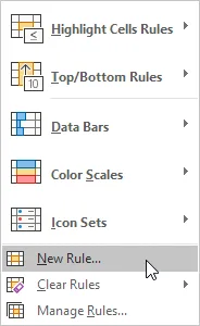
4. Click New Rule.
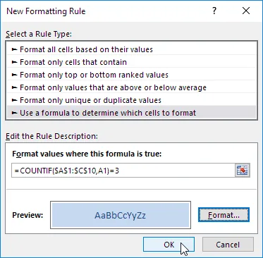
5. Choose a rule type: “Use a formula to determine which cells to format.”
6. Enter the formula =COUNTIF($A$1:$C$10,A1)=3
7. Select a formatting style and click OK.
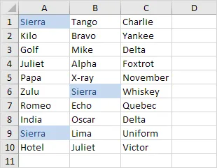
Result: Excel highlights the triplicate names.
Explanation: This formula =COUNTIF($A$1:$C$10, A1) checks the range A1:C10 and returns the number of cells that match the value in cell A1. If COUNTIF($A$1:$C$10,A1) = 3, Excel formats cell A1. Always type the formula in the first cell at the top-left of the range (A1:C10). Excel automatically fills the same formula into other cells. Therefore, Cell A2 has the formula =COUNTIF($A$1:$C$10,A2)=3. Cell A3 has =COUNTIF($A$1:$C$10,A3)=3, and so on. Here we use an absolute reference ($A$1:$C$10).
Note: You can use any formula you like. For Example, use =COUNTIF($A$1:$C$10, A1)>3 to highlight data that repeats more than 3 times.
💎 Identify Duplicate Rows in Excel
In Excel, COUNTIFS can be used to find and highlight duplicate rows instead of using COUNTIF.
1. Select the range A1:C10.
2. From the Home tab, find the Styles group. Then select Conditional Formatting options.
3. Click New Rule.
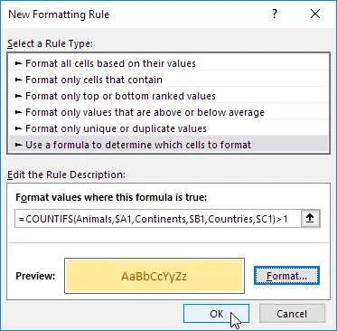
4. Now, choose a rule type: ‘Use a formula to determine which cells to format’.
5. Enter the formula =COUNTIFS(Animals,$A1,Continents,$B1,Countries,$C1)>1
6. Select a formatting style and click OK.
Note: The named range “Animals” covers A1 through A10, “Continents” covers B1 through B10, and “Countries” covers C1 through C10. =COUNTIFS(Animals,$A1, Continents,$B1, Countries,$C1) formula counts the number of rows that meet multiple criteria at the same time, such as Leopard in Africa and Zambia.
Result: Excel highlights the duplicate rows.
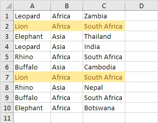
Explanation: If the formula COUNTIFS(Animals,$A1, Continents,$B1, Countries,$C1) > 1 finds more than one row with the same values (for example, Leopard, Africa, Zambia), Excel will apply formatting to cell A1. Always type the formula in the first cell of the range. In our case, it selects the first cell of the range (A1:C10). Excel applies the formula to other cells without extra work.
We fixed each column by adding a $ before the column letter ($A1, $B1, $C1). As a result, cells A1, B1, and C1 now have the same formula and cell A2, B2 and C2 contain the formula =COUNTIFS(Animals,$A2,Continents,$B2,Countries,$C2)>1, and so on.
💎 Remove Duplicates
In Excel, the Remove Duplicates tool allows you to quickly get rid of duplicate entries or rows. First, locate the Data Tools section from the Data tab. Then click on the Remove Duplicates option.

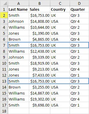
As shown below, Excel removes duplicate rows (blue) but keeps the first identical row it finds (yellow).
Note: Learn more about this useful Excel tool by visiting our page on removing duplicates.
6/10 Completed! Learn more about conditional formatting ➝
Next Chapter: Charts